See the Examples of our Articles
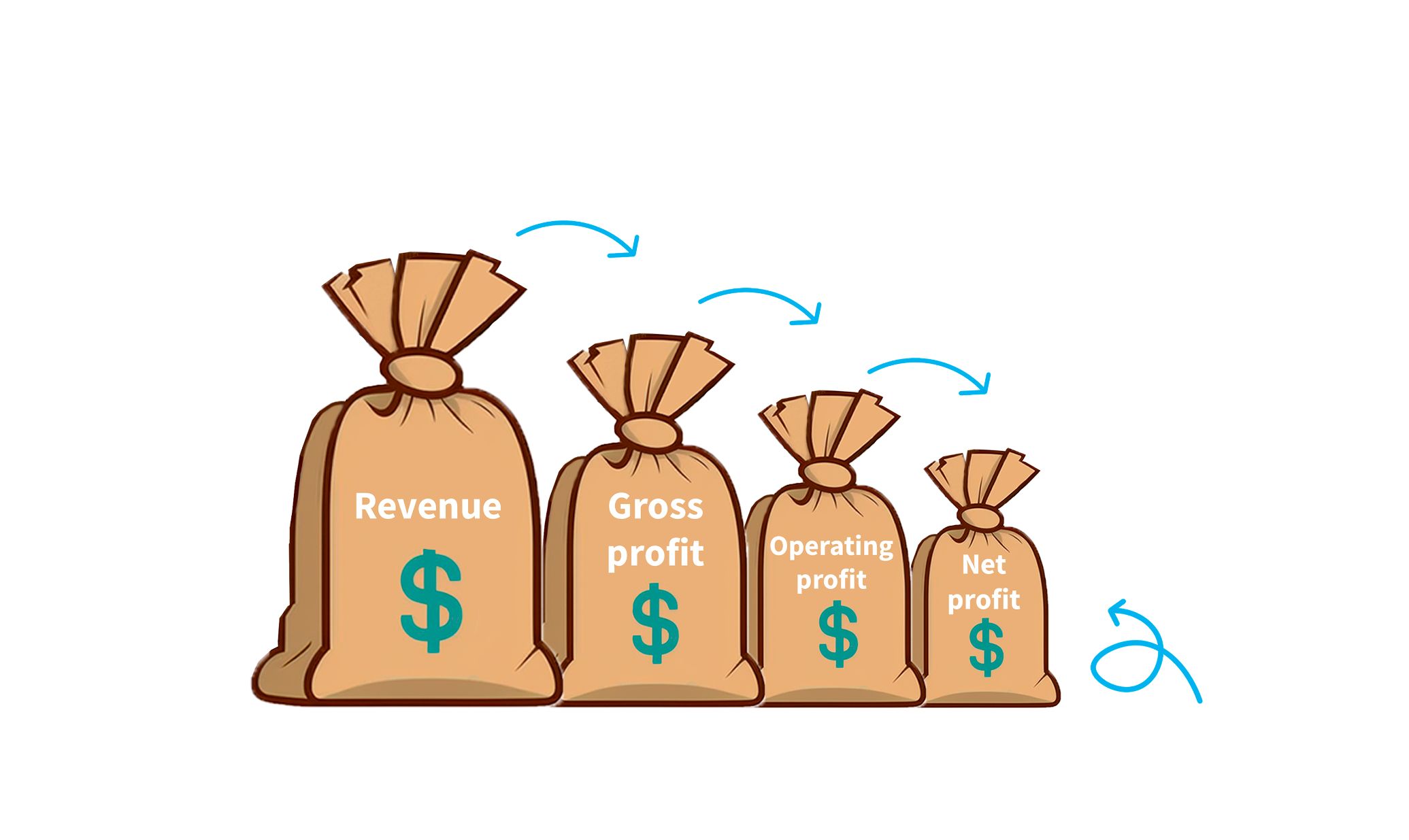
Understanding Profit
Learn the difference between gross profit and net profit, and how losses can affect businesses. Understand how to calculate profit and loss in business and finance
The Interpretation of Financial Statements
Learn to analyse a company by understanding their income statements, balance sheets, and ratios.